


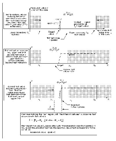
This example uses a bisectional search to find the minimum setup time for a D flip-flop. The circuit for this example is /bisect/dff_top.sp in the Star-Hspice $installdir/demo/hspice demonstration file directory. The files in Figures Bisection Example for Three Iterations and Transition at Minimum Setup Time show the results of this demo. Note that setup time is not optimized directly, but is extracted from its relationship with the DelayTime parameter (the time preceding the data signal), which is the parameter being optimized.
File: $installdir/demo/hspice/bisect/dff_top.sp
* DFF_top Bisection Search for Setup Time
*
* PWL Stimulus
*
v28 data gnd PWL
+ 0s 5v
+ 1n 5v
+ 2n 0v
+ Td = "DelayTime" $ Offsets Data from time 0 by DelayTime
v27 clock gnd PWL
+ 0s 0v
+ 3n 0v
+ 4n 5v
*
* Specify DelayTime as the search parameter and provide
* the lower and upper limits.
*
.PARAM DelayTime= Opt1 ( 0.0n, 0.0n, 5.0n )
*
* Transient simulation with Bisection Optimization
*
.TRAN 1n 8n Sweep Optimize = Opt1
+ Result = MaxVout $ Look at measure
+ Model = OptMod
*
* This measure finds the transition if it exists
*
.MEASURE Tran MaxVout Max v(D_Output) Goal = `v(Vdd)'
*
* This measure calculates the setup time value
*
.MEASURE Tran SetupTime Trig v(Data) Val = `v(Vdd)/2' Fall = 1
+ Targ v(Clock) Val = `v(Vdd)/2' Rise = 1
*
* Optimization Model
*
.MODEL OptMod Opt
+ Method = Bisection
.OPTIONS Post Brief NoMod
*************************************
* AvanLink to Cadence Composer by Avant!
* Hspice Netlist
* May 31 15:24:09 1994
*************************************
.MODEL nmos nmos LEVEL=2
.MODEL pmos pmos LEVEL=2
.Global vdd gnd
.SUBCKT XGATE control in n_control out
m0 in n_control out vdd pmos l=1.2u w=3.4u
m1 in control out gnd nmos l=1.2u w=3.4u
.ends
.SUBCKT INV in out wp=9.6u wn=4u l=1.2u
mb2 out in gnd gnd nmos l=l w=wn
mb1 out in vdd vdd pmos l=l w=wp
.ends
.SUBCKT DFF c d nc nq
Xi64 nc net46 c net36 XGATE
Xi66 nc net38 c net39 XGATE
Xi65 c nq nc net36 XGATE
Xi62 c d nc net39 XGATE
Xi60 net722 nq INV
Xi61 net46 net38 INV
Xi59 net36 net722 INV
Xi58 net39 net46 INV
c20 net36 gnd c=17.09f
c15 net39 gnd c=15.51f
c12 net46 gnd c=25.78f
c4 nq gnd c=25.28f
c3 net722 gnd c=19.48f
c16 net38 gnd c=16.48f
.ENDS
*-------------------------------------------------------------
* Main Circuit Netlist:
*-------------------------------------------------------------
v14 vdd gnd dc=5
c10 vdd gnd c=35.96f
c15 d_output gnd c=21.52f
c12 dff_nq gnd c=11.73f
c11 net31 gnd c=42.01f
c14 net27 gnd c=34.49f
c13 net25 gnd c=41.73f
c8 clock gnd c=5.94f
c7 data gnd c=7.93f
Xi3 net25 net31 net27 dff_nq DFF l=1u wn=3.8u wp=10u
Xi6 data net31 INV
Xi5 net25 net27 INV
Xi4 clock net25 INV
Xi2 dff_nq d_output INV wp=26.4u wn=10.6u
.END
The top plot in Transition at Minimum Setup Time shows the relationship between the clock and data pulses that determine the setup time. The bottom plot shows the output transition.
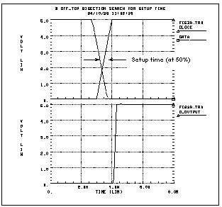
Find the actual value for the setup time in the "Optimization, Results" section of the Star-Hspice listing file:
optimization completed, the condition
relin = 1.0000E-03 is satisfied
**** optimized parameters opt1
.PARAM DelayTime =1.7188n
...
maxvout = 5.0049E+00 at= 4.5542E-09
from = .0000E+00 to= 8.0000E-09
setuptime= 2.8125E-10 targ= 3.5000E-09 trig= 3.2188E-09
This listing file excerpt shows that the optimal value for the setup time is 0.28125 nanoseconds.
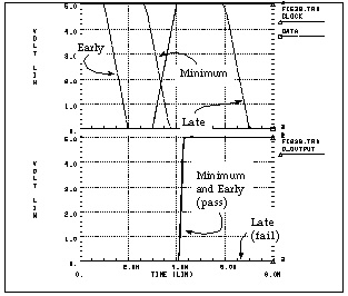
The top plot in Early, Minimum, and Late Setup and Hold Times shows examples of early and late data transitions, as well as the transition at the minimum setup time. The bottom plot shows how the timing of the data transition affects the output transition. These results were produced with the following analysis statement:
* Sweep 3 values for DelayTime Early Optim Late
*
.TRAN 1n 8n Sweep DelayTime Poi 3 0.0n 1.7188n 5.0n
This analysis produces the following results:
*** parameter DelayTime = .000E+00 *** $ Early
setuptime = 2.0000E-09 targ= 3.5000E-09 trig= 1.5000E-09
*** parameter DelayTime = 1.719E-09 *** $ Optimal
setuptime = 2.8120E-10 targ= 3.5000E-09 trig= 3.2188E-09
*** parameter DelayTime = 5.000E-09 *** $ Late
setuptime = -3.0000E-09 targ= 3.5000E-09 trig= 6.5000E-09Star-Hspice Manual - Release 2001.2 - June 2001