Understanding Bisection

Formerly, engineers built external drivers to submit multiple parameterized Star-Hspice jobs, with each job exploring a region of the operating envelope of the circuit. In addition, the driver needed to provide part of the analysis by post-processing the Star-Hspice results to deduce the limiting conditions.

Because characterization of circuits in this way is associated with small jobs, the individual analysis times are relatively small compared with the overall job time. This methodology is inefficient because of the overhead of submitting the job, reading and checking the netlist, and setting up the matrix. Efficiency in analyzing timing violations can be increased with more intelligent methods of determining the conditions causing timing failure. The bisection optimization method was developed to make cell characterization in Star-Hspice more efficient.

Star-Hspice bisection methodology saves time in three ways:

• Reduction of multiple jobs to a single characterization job
• Removal of post-processing requirements
• Use of accuracy-driven iteration

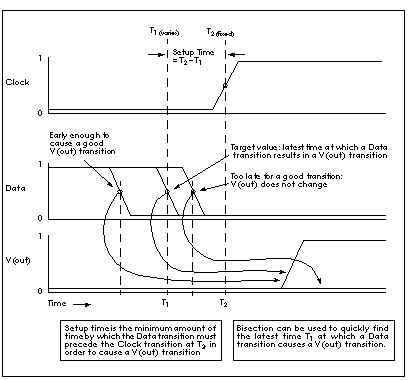
Determining Setup Time with Bisection Violation Analysis illustrates a typical analysis of setup time constraints. A cell is driven by clock and data input waveforms. There are two input transitions, rise and fall, that occur at times T 1 and T 2 . The result is an output transition, when V(out) goes from low to high. The following relationship between times T 1 (data) and T 2 (clock) must be true in order for the V(out) transition to occur:

T 2 > (T 1 + setup time)

The goal of the characterization, or violation analysis, is to determine the setup time. This is done by keeping T 2 fixed while repeating the simulation with different values of T 1 and observing which T 1 values produce the output transition and which values do not.

Previously, it was necessary to do very tight sweeps of the delay between the data setup and clock edge, looking for the value at which the transition fails to occur. This was done by sweeping a value that specifies how far the data edge precedes a fixed clock edge. This methodology is time consuming, and is not accurate unless the sweep step is very small. The setup time value cannot be determined accurately by linear search methods unless extremely small steps from T 1 to T 2 are used to simulate the circuit at each point while monitoring the outcome.

For example, even if it is known that the desired transition occurs during a particular five nanosecond period, searching for the actual setup time to within 0.1 nanoseconds over that five nanosecond period takes as many as 50 simulations. Even after this, the error in the result can be as large as 0.05 nanoseconds.

Figure 30-1: Determining Setup Time with Bisection Violation Analysis

The Star-Hspice bisection feature greatly reduces the amount of work and computational time required to find an accurate solution to this type of problem. The following pages show examples of using this feature to identify setup, hold, and minimum clock pulse width timing violations.