There are two forms of the Star-Hspice LAPLACE function call, one for transconductance and one for voltage gain transfer functions. See Using G and E Elements for the general forms and Element Statement Parameters for descriptions of the parameters.
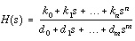
To use the Star-Hspice LAPLACE modeling function, you must find the k0, ..., kn and d0, ..., dm coefficients of the transfer function. The transfer function is the s-domain (frequency domain) ratio of the output of a single-source circuit to the input, with initial conditions set to zero. The Laplace transfer function is represented by:
where s is the complex frequency j2 f, Y(s) is the Laplace transform of the output signal, and X(s) is the Laplace transform of the input signal.
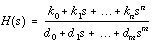
The general form of the transfer function H(s) in the frequency domain is:
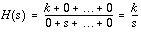
The order of the numerator of the transfer function cannot be greater than the order of the denominator, except for differentiators, for which the transfer function H(s) = ks. All of the transfer function's k and d coefficients can be parameterized in the Star-Hspice circuit descriptions.
The first step in determining the transfer function of a circuit is to convert the circuit to the s-domain by transforming each element's value into its s-domain equivalent form.
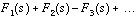
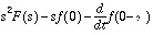
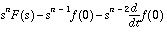
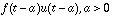
Tables Laplace Transforms for Common Source Functions and Laplace Transforms for Common Operations show transforms used to convert some common functions to the s-domainNillson, James W. Electric Circuits, 4th Edition. Reading, Massachusetts: Addison-Wesley, 1993.
|
||
u(t) |
||
t |
||
e
|
||
sin
|
||
cos
|
||
|
|
||
|
|
||
|
|
||
|
|
||
te-at |
||
|
|
||
|
|
|
|
|
|
|
|
|
|
|
|
|
|
|
|
|
|
|
|
|
|
|
|
|
|
|
|
|
|
|
|
|
|
|
|
|
|
|
|
The following examples describe how to determine the appropriate coefficients for the Laplace modeling function call in Star-Hspice.
To find the voltage gain transfer function for the circuit in LAPLACE Example 1 Circuit, convert the circuit to its equivalent s-domain circuit and solve for vo / vg.
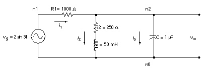
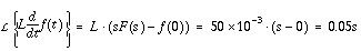
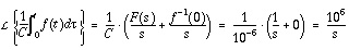
Use transforms from Laplace Transforms for Common Operations to convert the inductor, capacitor, and resistors. L{f(t)} represents the Laplace transform of f(t):
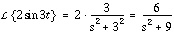
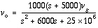
To convert the voltage source to the s-domain, use the sin  t transform from Laplace Transforms for Common Source Functions:
S-Domain Equivalent of the LAPLACE Example 1 Circuit displays the s-domain equivalent circuit.
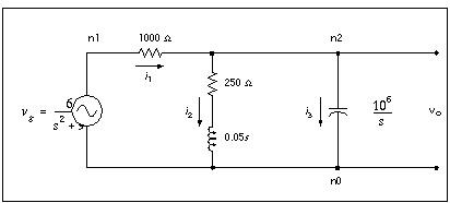
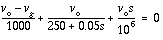
Summing the currents leaving node n2:
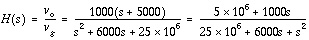
The voltage gain transfer function is:
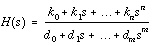
For the Star-Hspice Laplace function call, use kn and dm coefficients for the transfer function in the form:
The coefficients from the voltage gain transfer function above are:
Using these coefficients, a Star-Hspice Laplace modeling function call for the voltage gain transfer function of the circuit in LAPLACE Example 1 Circuit is:
Eexample1 n1 n0 LAPLACE n2 n0 5E6 1000 / 25E6 6000 1
You can model a differentiator using either G or E Elements as shown in the following example.
For a differentiator, the voltage gain transfer function is:
In the general form of the transfer function,
If you set k1 = k and d0 = 1 and the remaining coefficients are zero, then the equation becomes:
Using the coefficients k1 = k and d0 = 1 in the Laplace modeling, the Star-Hspice circuit descriptions for the differentiator are:
Edif out GND LAPLACE in GND 0 k / 1
Gdif out GND LAPLACE in GND 0 k / 1
An integrator can be modeled by G or E Elements as follows:
For an integrator, the voltage gain transfer function is:
In the general form of the transfer function:
Like the previous example, if you make k0 = k and d1 = 1, then the equation becomes:
This section describes the general form of the pole/zero transfer function and provides examples of converting specific transfer functions into pole/zero circuit descriptions.
The POLE function in Star-Hspice is useful when the poles and zeros of the circuit are available. The poles and zeros can be derived from the transfer function, as described in this chapter, or you can use the Star-Hspice .PZ statement to find them, as described in .PZ (Pole/Zero) Statement.
There are two forms of the Star-Hspice LAPLACE function call, one for transconductance and one for voltage gain transfer functions. See Using G and E Elements for the general forms and list of optional parameters.
To use the POLE pole/zero modeling function, find the a, b, f, and  coefficients of the transfer function. The transfer function is the s-domain (frequency domain) ratio of the output of a single-source circuit to the input, with initial conditions set to zero.
The general expanded form of the pole/zero transfer function H(s) is:
The a, b,  , and f values can be parameterized.
Ghigh_pass 0 out POLE in 0 1.0 0.0,0.0 / 1.0 0.001,0.0
Elow_pass out 0 POLE in 0 1.0 / 1.0, 1.0,0.0 0.5,0.1379
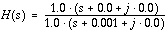
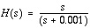
The Ghigh_pass statement describes a high pass filter with transfer function:
The Elow_pass statement describes a low-pass filter with transfer function:
To write a Star-Hspice pole/zero circuit description for an element, you need to know the element's transfer function H(s) in terms of the a, b, f, and  coefficients. Use the values of these coefficients in POLE function calls in the Star-Hspice circuit description.
First, however, simplify the transfer function, as described in the next section.
Complex poles and zeros occur in conjugate pairs (a set of complex numbers differ only in the signs of their imaginary parts):
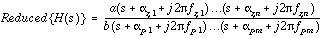
To write the transfer function in Star-Hspice pole/zero format, supply coefficients for one term of each conjugate pair and Star-Hspice provides the coefficients for the other term. If you omit the negative complex roots, the result is the reduced form of the transfer function, Reduced{H(s)}. Find the reduced form by collecting all the general form terms with negative complex roots:
Then discard the right-hand term, which contains all the terms with negative roots. What remains is the reduced form:
For this function find the a, b, f, and  coefficients to use in a Star-Hspice POLE function for a voltage gain transfer function. The following examples show how to determine the coefficients and write POLE function calls for a high-pass filter and a low-pass filter.
For a high-pass filter with a given transconductance transfer function, such as:
Find the a, b,  , and f coefficients necessary to write the transfer function in the general form (1) shown previously, so that you can clearly see the conjugate pairs of complex roots. You only need to supply one of each conjugate pair of roots in the Laplace function call. Star-Hspice automatically inserts the other root.
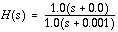
To get the function into a form more similar to the general form of the transfer function, rewrite the given transconductance transfer function as:
Since this function has no negative imaginary parts, it is already in the Star-Hspice reduced form (2) shown previously. Now you can identify the a, b, f, and  coefficients so that the transfer function H(s) matches the reduced form. This matching process obtains the following values:
Using these coefficients in the reduced form provides the desired transfer function,  .
.
So the general transconductance transfer function POLE function call,
Gxxx n+ n- POLE in+ in- az1,fz1...
zn,fzn / b
p1,fp1...
pm,fpm
for an element named Ghigh_pass becomes:
Ghigh_pass gnd out POLE in gnd 1.0 0.0,0.0 / 1.0 0.001,0.0
For a low-pass filter with the given voltage gain transfer function:
you need to find the a, b,  , and f coefficients to write the transfer function in the general form, so that you can identify the complex roots with negative imaginary parts.
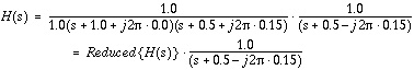
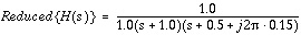
To separate the reduced form, Reduced{H(s)}, from the terms with negative imaginary parts, rewrite the given voltage gain transfer function as:
Now assign coefficients in the reduced form to match the given voltage transfer function. The following coefficient values produce the desired transfer function:
a =1.0 b = 1.0  p1 = 1.0 fp1 = 0
  p2 = 0.5 fp2 = 0.15
These coefficients can be substituted in the POLE function call for a voltage gain transfer function:
Exxx n+ n- POLE in+ in- az1,fz1...
zn,fzn / b
p1,fp1...
pm,fpm
for an element named Elow_pass to obtain the Star-Hspice statement:
Elow_pass out GND POLE in 1.0 / 1.0 1.0,0.0 0.5,0.15
Most RC lines can have very simple models, with just a single dominant pole. The dominant pole can be found by AWE methods, computed based on the total series resistance and capacitanceGhausi, Kelly, and M.S. On the Effective Dominant Pole of the Distributed RC Networks. Jour. Franklin Inst., June 1965, pp. 417- 429., or determined by the Elmore delayElmore, W.C. and Sands, M. Electronics, National Nuclear Energy Series, New York: McGraw-Hill, 1949..
The Elmore delay uses the value (d1-k1) as the time constant of a single-pole approximation to the complete H(s), where H(s) is the transfer function of the RC network to a given output. The inverse Laplace transform of h(t) is H(s):
Actually, the Elmore delay is the first moment of the impulse response, and so corresponds to a first order AWE result.
* Laplace testing RC line
.Tran 0.02ns 3ns
.Options Post Accurate List Probe
v1 1 0 PWL 0ns 0 0.1ns 0 0.3ns 5 1.3ns 5 1.5ns 0
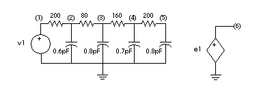
r1 1 2 200
c1 2 0 0.6pF
r2 2 3 80
c2 3 0 0.8pF
r3 3 4 160
c3 4 0 0.7pF
r4 4 5 200
c4 5 0 0.8pF
e1 6 0 LAPLACE 1 0 1 / 1 1.16n
.Probe v(1) v(5) v(6)
.Print v(1) v(5) v(6)
.End
The output of the RC circuit shown in Circuits for an RC Line can be closely approximated by a single pole response, as shown in Transient Response of the RC Line and Single-Pole Approximation.
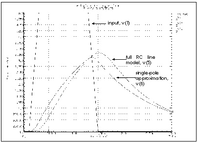
Notice in Transient Response of the RC Line and Single-Pole Approximation that the single pole approximation has less delay: 1 ns compared to 1.1 ns for the full RC line model at 2.5 volts. The single pole approximation also has a lower peak value than the RC line model. All other things being equal, a circuit with a shorter time constant results in less filtering and allows a higher maximum voltage value. The single-pole approximation produces a lower amplitude and less delay than the RC line because the single pole neglects the other three poles in the actual circuit. However, a single-pole approximation still gives very good results for many problems.
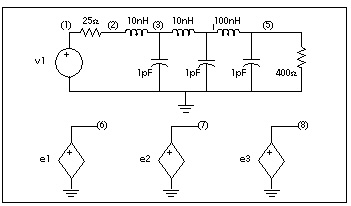
Single-pole transfer function approximations can cause larger errors for low-loss lines than for RC lines since lower resistance allows ringing. Because circuit ringing creates complex pole pairs in the transfer function approximation, at least one complex pole pair is needed to represent low-loss line response. Circuits for a Low-Loss Line shows a typical low-loss line, along with the transfer function sources used to test the various approximations. The transfer functions were obtained by asymptotic waveform evaluationPillage, L.T. and Rohrer, R.A. Asymptotic Waveform Evaluation for Timing Analysis, IEEE Trans. CAD, Apr. 1990, pp. 352 - 366..
* Laplace testing LC line Pillage Apr 1990
.Tran 0.02ns 8ns
.Options Post Accurate List Probe
v1 1 0 PWL 0ns 0 0.1ns 0 0.2ns 5
r1 1 2 25
L1 2 3 10nH
c2 3 0 1pF
L2 3 4 10nH
c3 4 0 1pF
L3 4 5 100nH
c4 5 0 1pF
r4 5 0 400
e3 8 0 LAPLACE 1 0 0.94 / 1.0 0.6n
e2 7 0 LAPLACE 1 0 0.94e20 / 1.0e20 0.348e11 14.8 1.06e-9 2.53e-19
+ SCALE=1.0e-20
e1 6 0 LAPLACE 1 0 0.94 / 1 0.2717e-9 0.12486e-18
.Probe v(1) v(5) v(6) v(7) v(8)
.Print v(1) v(5) v(6) v(7) v(8)
.End
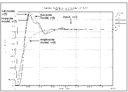
Transient Response of the Low-Loss Line shows the transient response of the low-loss line, along with E Element Laplace models using one, two, and four polesPillage, L.T. and Rohrer, R.A. Asymptotic Waveform Evaluation for Timing Analysis, IEEE Trans. CAD, Apr. 1990, pp. 352 - 366.. Note that the single-pole model shows none of the ringing of the higher order models. Also, all of the E models had to adjust the gain of their response for the finite load resistance, so the models are not independent of the load impedance. The 0.94 gain multiplier in the models takes care of the 25 ohm source and 400 ohm load voltage divider. All of the approximations give good delay estimations.
While the two-pole approximation gives reasonable agreement with the transient overshoot, the four-pole model gives almost perfect agreement. The actual circuit has six poles. Scaling was used to bring some of the very small numbers in the Laplace model above the 1e-28 limit of Star-Hspice. The SCALE parameter multiplies every parameter in the LAPLACE specification by the same value, in this case 1.0E-20.
A low-loss line allows reflections between the load and source, while the loss of an RC line usually isolates the source from the load. So you can either incorporate the load into the AWE transfer function approximation or create a Star-Hspice model that allows source/load interaction. If you allow source/load interaction, the AWE expansions do not have to be done each time you change load impedances, allowing you to handle nonlinear loads and remove the need for a gain multiplier, as in the circuit file shown. You can use four voltage controlled current sources, or G Elements, to create a Y parameter model for a transmission line. The Y parameter network allows the source/load interaction needed. The next example shows such a Y parameter model for a low-loss line.
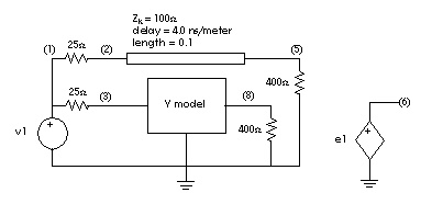
A model that is independent of load impedance is more complicated. You can still use AWE techniques, but you need a way for the load voltage and current must be able to interact with the source impedance. Given a transmission line of 100 ohms and 0.4 ns total delay, as shown in Line and Y Parameter Modeling, compare the response of the line using a Y parameter model and a single-pole model.
The voltage and current definitions for a Y parameter model are shown in Y Matrix for the Two-Port Network.
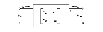
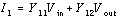
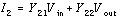
The general network in Y Matrix for the Two-Port Network is described by the following equations, which can be translated into G Elements:
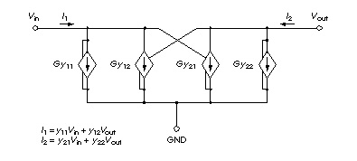
A schematic for a set of two-port Y parameters is shown in Schematic for the Y Parameter Network. Note that the circuit is essentially composed of G Elements.
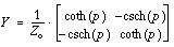
The Laplace parameters for the Y parameter model are determined by a Pade expansion of the Y parameters of a transmission line, as shown in matrix form in the following equation.
where p is the product of the propagation constant and the line lengthKuo, F. F. Network Analysis and Synthesis. John Wiley and Sons, 1966..
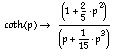
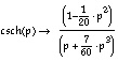
A Pade approximation contains polynomials in both the numerator and the denominator. Since a Pade approximation can model both poles and zeros and since coth and csch functions also contain both poles and zeros, a Pade approximation gives a better low order model than a series approximation. A Pade expansion of coth(p) and csch(p), with second order numerator and third order denominator, is given below:
When you substitute ( ) for p, you get polynomial expressions for each G Element. When you substitute 400 nH for L, 40 pF for C, 0.1 meter for length, and 100 for Zo (
 ) in the matrix equation above, you get values you can use in a circuit file.
The circuit file shown below uses all of the above substitutions. The Pade approximations have different denominators for csch and coth, but the circuit file contains identical denominators. Although the actual denominators for csch and coth are only slightly different, using them would cause oscillations in the Star-Hspice response. To avoid this problem, use the same denominator in the coth and csch functions in the example. The simulation results may vary, depending on which denominator is used as the common denominator, because the coefficient of the third order term is changed (but by less than a factor of 2).
* Laplace testing LC line Pade
.Tran 0.02ns 5ns
.Options Post Accurate List Probe
v1 1 0 PWL 0ns 0 0.1ns 0 0.2ns 5
r1 1 2 25
r3 1 3 25
u1 2 0 5 0 wire1 L=0.1
r4 5 0 400
r8 8 0 400
e1 6 0 LAPLACE 1 0 1 / 1 0.4n
Gy11 3 0 LAPLACE 3 0 320016 0.0 2.048e-14 / 0.0 0.0128 0.0 2.389e-22
Gy12 3 0 LAPLACE 8 0 -320016 0.0 2.56e-15 / 0.0 0.0128 0.0 2.389e-22
Gy21 8 0 LAPLACE 3 0 -320016 0.0 2.56e-15 / 0.0 0.0128 0.0 2.389e-22
Gy22 8 0 LAPLACE 8 0 320016 0.0 2.048e-14 / 0.0 0.0128 0.0 2.389e-22
.model wire1 U Level=3 PLEV=1 ELEV=3 LLEV=0 MAXL=20
+ ZK=100 DELAY=4.0n
.Probe v(1) v(5) v(6) v(8)
.Print v(1) v(5) v(6) v(8)
.End
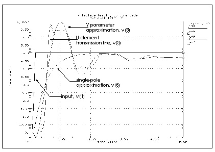
Transient Response of the Y Parameter Line Model compares the output of the Y parameter model with that of a full transmission line simulation and with that obtained for a single pole transfer function. In the latter case, the gain was not corrected for the load impedance, so the function produces an incorrect final voltage level. As expected, the Y parameter model gives the correct final voltage level. Although the Y parameter model gives a good approximation of the circuit delay, it contains too few poles to model the transient details fully. However, the Y parameter model does give excellent agreement with the overshoot and settling times.
This example simulates a ninth order low-pass filter circuit and compares the results with its equivalent pole/zero description using an E Element. The results are identical, but the pole/zero model runs about 40% faster. The total CPU times for the two methods are shown in Simulation Time Summary. For larger circuits, the computation time saving can be much higher.
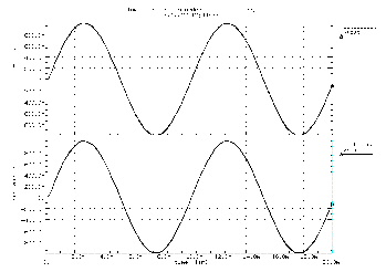
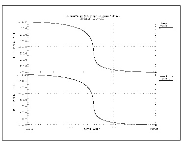
The input listings for each model type are shown below. Figures Transient Responses of the Circuit and Pole/Zero Models and AC Analysis Responses of the Circuit and Pole/Zero Models display the transient and frequency response comparisons resulting from the two modeling methods.
low_pass9a.sp 9th order low_pass filter.
* Reference: Jiri Vlach and Kishore Singhal, "Computer Methods for
* Circuit Analysis and Design", Van Nostrand Reinhold Co., 1983,
* pages 142, 494-496.
*
.PARAM freq=100 tstop='2.0/freq'
*.PZ v(out) vin
.AC dec 50 .1k 100k
.OPTIONS dcstep=1e3 post probe unwrap
.PROBE ac vdb(out) vp(out)
.TRAN STEP='tstop/200' STOP=tstop
.PROBE v(out)
vin in GND sin(0,1,freq) ac 1
.SUBCKT fdnr 1 r1=2k c1=12n r4=4.5k
r1 1 2 r1
c1 2 3 c1
r2 3 4 3.3k
r3 4 5 3.3k
r4 5 6 r4
c2 6 0 10n
eop1 5 0 opamp 2 4
eop2 3 0 opamp 6 4
.ENDS
*
rs in 1 5.4779k
r12 1 2 4.44k
r23 2 3 3.2201k
r34 3 4 3.63678k
r45 4 out 1.2201k
c5 out 0 10n
x1 1 fdnr r1=2.0076k c1=12n r4=4.5898k
x2 2 fdnr r1=5.9999k c1=6.8n r4=4.25725k
x3 3 fdnr r1=5.88327k c1=4.7n r4=5.62599k
x4 4 fdnr r1=1.0301k c1=6.8n r4=5.808498k
.END
ninth.sp 9th order low_pass filter.
.PARAM twopi=6.2831853072
.PARAM freq=100 tstop='2.0/freq'
.AC dec 50 .1k 100k
.OPTIONS dcstep=1e3 post probe unwrap
.PROBE ac vdb(outp) vp(outp)
.TRAN STEP='tstop/200' STOP=tstop
.PROBE v(outp)
vin in GND sin(0,1,freq) ac 1
Epole outp GND POLE in GND 417.6153
+ 0. 3.8188k
+ 0. 4.0352k
+ 0. 4.7862k
+ 0. 7.8903k / 1.0
+ '73.0669*twopi' 3.5400k
+ '289.3438*twopi' 3.4362k
+ '755.0697*twopi' 3.0945k
+ '1.5793k*twopi' 2.1105k
+ '2.1418k*twopi' 0.
repole outp GND 1e12
.END
Circuit model simulation times:
analysis time # points . iter conv.iter
op point 0.23 1 3
ac analysis 0.47 151 151
transient 0.75 201 226 113 rev= 0
readin 0.22
errchk 0.13
setup 0.10
output 0.00
total cpu time 1.98 seconds
Pole/zero model simulation times:
analysis time # points tot. iter conv.iter
op point 0.12 1 3
ac analysis 0.22 151 151
transient 0.40 201 222 111 rev= 0
readin 0.23
errchk 0.13
setup 0.02
output 0.00
total cpu time 1.23 seconds
 ,
,
 { f(t) }= F(s)
 (t)
(t)


 t
t
 t
t


 { f(t) } = F(s)


 (u is the step function)


 ,
, 


 (1)
(1)

 , for poles
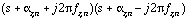 , for zeros
 (2)
(2)
 z1 = 0.0 fz1 = 0.0
 p1 = 0.001 fp1 = 0.0


 ,
,