Input Netlist File Composition

Title of Simulation and .TITLE Statement

The simulation title is set using the first line of the input file. This line is always read and used as the title of the simulation regardless of the contents of this line. The title is printed verbatim in each section heading of the output listing file of the simulation.

The .TITLE statement, as shown in the first syntax below, can be used on the first line of the netlist to set the title, although the .TITLE syntax is not necessary. In the second form shown below, the string is the first line of the input file. The first line of the input file is always the implicit title. If a Star-Hspice statement appears as the first line in a file, it is interpreted as a title and is not executed.

An .ALTER statement does not support the usage of .TITLE. To change a title for a .ALTER statement, place the title content in the .ALTER statement itself.

Syntax

.TITLE <string of up to 72 characters>

or

<string of up to 72 characters>

Comments

An asterisk (*) as the first nonblank character or an inline dollar sign ($) indicates a comment statement.

Syntax

* <comment on a line by itself>

or

<HSPICE statement> $ <comment following HSPICE input>

Example

*RF = 1K GAIN SHOULD BE 100

$ MAY THE FORCE BE WITH MY CIRCUIT

VIN 1 0 PL 0 0 5V 5NS $ 10v 50ns

R12 1 0 1MEG $ FEED BACK

You can place comment statements anywhere in the circuit description.

The * must be in the first space on the line.

The $ must be used for comments that do not begin at the first space on a line (for example, for comments that follow Star-Hspice input on the same line). The $ must be preceded by a space or comma if it is not the first nonblank character. The $ is allowed within node or element names.

Element and Source Statements

Element statements describe the netlists of devices and sources. Elements are connected to one another by nodes, which can either be numbers or names. Element statements specify

• Type of device
• Nodes to which the device is connected
• Parameter values that describe the operating electrical characteristics of the device

Element statements also can reference model statements that define the electrical parameters of the element.

Element statements for the various types of Star-Hspice elements are described in the chapters on those types of elements.

Syntax

elname <node1 node2 ... nodeN> <mname>
+ <pname1 = val1> <pname2 = val2> <M = val>

or

elname < node1 node2 ... nodeN > < mname >
+ < pname = 'expression' > < M = val >

or

elname <node1 node2 ... nodeN> <mname>
+ <val1 val2 ... valn>

where:

Example

Q1234567 4000 5000 6000 SUBSTRATE BJTMODEL AREA = 1.0

The previous example specifies a bipolar junction transistor with its collector connected to node 4000, its base connected to node 5000, its emitter connected to node 6000, and its substrate connected to node SUBSTRATE. The transistor parameters are described in the model statement referenced by the name BJTMODEL.

M1 ADDR SIG1 GND SBS N1 10U 100U

The previous example specifies a MOSFET called M1, whose drain, gate, source, and substrate nodes are named ADDR, SIG1, GND, and SBS, respectively. The element statement calls an associated model statement, N1. MOSFET dimensions are specified as width = 100 microns and length = 10 microns.

M1 ADDR SIG1 GND SBS N1 w1+w l1+l

The previous example specifies a MOSFET called M1, whose drain, gate, source, and substrate nodes are named ADDR, SIG1, GND, and SBS, respectively. The element statement calls an associated model statement, N1. MOSFET dimensions are also specified as algebraic expressions, width = w1+w and length = l1+l.

.SUBCKT or .MACRO Statement

The syntax is:

.SUBCKT subnam n1 < n2 n3 ...> < parnam = val ...>

or

.MACRO subnam n1 < n2 n3 ... > < parnam = val ...>

where:

subnam Specifies reference name for the subcircuit model call

n1 ... Node numbers for external reference; cannot be ground node (zero). Any element nodes appearing in the subcircuit but not included in this list are strictly local, with three exceptions:

1. the ground node (zero)

2. nodes assigned using BULK = node in the MOSFET or BJT models

3. nodes assigned using the .GLOBAL statement

parnam A parameter name set to a value. For use only in the subcircuit, overridden by an assignment in the subcircuit call or by a value set in a .PARAM statement.

Example

*FILE SUB2.SP TEST OF SUBCIRCUITS

.OPTIONS LIST ACCT

*

V1 1 0 1

.PARAM P5 = 5 P2 = 10

*

.SUBCKT SUB1 1 2 P4 = 4

R1 1 0 P4

R2 2 0 P5

X1 1 2 SUB2 P6 = 7

X2 1 2 SUB2

.ENDS

*

.MACRO SUB2 1 2 P6 = 11

R1 1 2 P6

R2 2 0 P2

.EOM

*

X1 1 2 SUB1 P4 = 6

X2 3 4 SUB1 P6 = 15

X3 3 4 SUB2

*

.MODEL DA D  CJA = CAJA CJP = CAJP VRB = -20 IS = 7.62E-18

+   PHI = .5 EXA = .5 EXP = .33

*

.PARAM CAJA = 2.535E-16 CAJP = 2.53E-16

.END

The above example defines two subcircuits: SUB1 and SUB2. These are resistor divider networks whose resistance values have been parameterized. They are called with the X1, X2, and X3 statements. Since the resistor value parameters are different in each call, these three calls produce different subcircuits.

.ENDS or .EOM Statement

The syntax is:

.ENDS <SUBNAM>

or

.EOM <SUBNAM>

Example

.ENDS OPAMP

.EOM MAC3

This statement must be the last for any subcircuit definition. The subcircuit name, if included, indicates which definition is being terminated. Subcircuit references (calls) may be nested within subcircuits.

Subcircuit Call Statement

The syntax is:

Xyyy n1 <n2 n3 ...> subnam <parnam = val ...> <M = val>

where:

Xyyy Subcircuit element name. Must begin with an "X", which may be followed by up to 15 alphanumeric characters.

n1 ... Node names for external reference

subnam Subcircuit model reference name

parnam A parameter name set to a value (val) for use only in the subcircuit. It overrides a parameter value assigned in the subcircuit definition, but is overridden by a value set in a .PARAM statement.

M Multiplier. Makes the subcircuit appear as M subcircuits in parallel. This is useful in characterizing circuit loading. No additional calculation time is needed to evaluate multiple subcircuits.

Example

X1 2 4 17 31 MULTI WN = 100 LN = 5

The above example calls a subcircuit model named MULTI. It assigns the parameters WN = 100 and LN = 5 to the parameters WN and LN given in the .SUBCKT statement (not shown). The subcircuit name is X1. All subcircuit names must begin with X.

Example

	.SUBCKT YYY NODE1 NODE2 VCC = 5V

	.IC NODEX = VCC

	R1 NODE1 NODEX 1

	R2 NODEX NODE2 1

	.EOM

	XYYY 5 6 YYY VCC = 3V

The above example defines a subcircuit named YYY. The subcircuit consists of two 1 ohm resistors in series. The subcircuit node, NODEX, is initialized with the .IC statement through the passed parameter VCC.

Element and Node Naming Conventions

Node Names

Nodes are the points of connection between elements in the input netlist file. In Star-Hspice, nodes are designated by either names or by numbers. Node numbers can be from 1 to 999999999999999; node number 0 is always ground. Letters that follow numbers in node names are ignored. Node names must begin with a letter and are followed by up to 1023 characters.

In addition to letters and digits, the following characters are allowed in node names:

Braces, "{ }", are allowed in node names, but Star-Hspice changes them to square brackets, "[ ]".

The following are not allowed in node names:

The period is reserved for use as a separator between the subcircuit name and the node name:

<subcircuitName>.<nodeName> .

The sorting order for operating point nodes is

a-z, !, #, $, %, *, +, -, /

Instance and Element Names

Star-Hspice elements have names that begin with a letter designating the element type, followed by up to 1023 alphanumeric characters. Element type letters are R for resistor, C for capacitor, M for a MOSFET device, and so on (see Element and Source Statements).

Subcircuit Node Names

Subcircuit node names are assigned two different names in Star-Hspice. The first name is assigned by concatenating the circuit path name with the node name through the (.) extension - for example, X1.XBIAS.M5.

The second subcircuit node name is a unique number that Star-Hspice assigns automatically to an input netlist file subcircuit. This number is concatenated using the ( : ) extension with the internal node name, giving the entire subcircuit's node name (for example, 10:M5). The node name is cross referenced in the output listing file Star-Hspice produces.

The ground node must be indicated by either the number 0, the name GND, or !GND. Every node should have at least two connections, except for transmission line nodes (unterminated transmission lines are permitted) and MOSFET substrate nodes (which have two internal connections). Floating power supply nodes are terminated with a 1 megohm resistor and a warning message.

Path Names of Subcircuit Nodes

A path name consists of a sequence of subcircuit names, starting at the highest level subcircuit call and ending at an element or bottom level node. The subcircuit names are separated by periods in the path name. The maximum length of the path name, including the node name, is 1024 characters.

You can use path names in the .PRINT, .PLOT, .NODESET, and .IC statements as an alternative method to reference internal nodes (nodes not appearing on the parameter list). Any node, including any internal node, can be referenced by its path name. Subcircuit node and element names follow the rules illustrated in Subcircuit Calling Tree with Circuit Numbers and Instance Names.

Figure 3-1: Subcircuit Calling Tree with Circuit Numbers and Instance Names

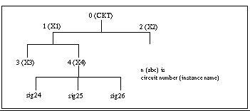
The path name of the node named sig25 in subcircuit X4 in Subcircuit Calling Tree with Circuit Numbers and Instance Names is X1.X4.sig25. You can use this path in Star-Hspice statements such as:

.PRINT v(X1.X4.sig25)

Abbreviated Subcircuit Node Names

You can use circuit numbers as an alternative to path names to reference nodes or elements in .PRINT, .PLOT, .NODESET, or .IC statements. Star-Hspice assigns a circuit number to all subcircuits on compilation, creating an abbreviated path name:

<subckt-num>:<name>

Every occurrence of a node or element in the output listing file is prefixed with the subcircuit number and colon. For example, 4:INTNODE1 denotes a node named INTNODE1 in a subcircuit assigned the number 4.

Any node not in a subcircuit is prefixed by 0: (0 references the main circuit). All nodes and subcircuits are identified in the output listing file with a circuit number referencing the subcircuit where the node or element appears. Abbreviated path names allow use of DC operating point node voltage output as input in a .NODESET for a later run; the part of the output listing titled "Operating Point Information" can be copied or typed directly into the input file, preceded by a .NODESET statement. This eliminates recomputing the DC operating point in the second simulation.

Automatic Node Name Generation

Star-Hspice has an automatic system for assigning internal node names. You can check both nodal voltages and branch currents by printing or plotting with the assigned node name. Several special cases for node assignment occur in Star-Hspice. Node 0 is automatically assigned as a ground node.

For CSOS (CMOS Silicon on Sapphire), if the bulk node is assigned the value -1, the name of the bulk node is B#. Use this name for printing the voltage at the bulk node. When printing or plotting current, for example .PLOT I(R1), Star-Hspice inserts a zero-valued voltage source. This source inserts an extra node in the circuit named Vnn, where nn is a number automatically generated by Star-Hspice and appears in the output listing file.

.GLOBAL Statement

The .GLOBAL statement globally assigns a node name. This means that all references to a global node name used at any level of the hierarchy in the circuit, will be connected to the same node.

The .GLOBAL statement is most often used when subcircuits are included in a netlist file. This statement assigns a common node name to subcircuit nodes. Power supply connections of all subcircuits are often assigned using a .GLOBAL statement. For example, .GLOBAL VCC connects all subcircuits with the internal node name VCC. Ordinarily, in a subcircuit the node name is given as the circuit number concatenated to the node name. When a .GLOBAL statement is used, the node name is not concatenated with the circuit number and is only assigned the global name. This allows exclusion of the power node name in the subcircuit or macro call.

Syntax

.GLOBAL node1 node2 node3 ...

where:

Example

This example shows global definitions for the nodes VDD and input_sig.

.GLOBAL VDD input_sig

.TEMP Statement

The temperature of a circuit for a Star-Hspice run is specified with the .TEMP statement or with the TEMP parameter in the .DC, .AC, and .TRAN statements. The circuit simulation temperature set by either of these is compared against the reference temperature set by the TNOM control option. The difference between the circuit simulation temperature and the reference temperature, TNOM, is used in determining the derating factors for component values. Temperature analysis is discussed in Temperature Analysis.

Syntax

.TEMP t1 <t2 <t3 ...>>

where:

Example

.TEMP -55.0 25.0 125.0

The .TEMP statement sets the circuit temperatures for the entire circuit simulation. Star-Hspice uses the temperature set in the .TEMP statement, along with the TNOM option setting (or the TREF model parameter) and the DTEMP element temperature, and simulates the circuit with individual elements or model temperatures.

Example

.TEMP 100
D1 N1 N2 DMOD DTEMP = 30
D2 NA NC DMOD
R1 NP NN 100 TC1 = 1 DTEMP = -30
.MODEL DMOD D IS = 1E-15 VJ = 0.6 CJA = 1.2E-13 CJP = 1.3E-14 TREF = 60.0

The circuit simulation temperature is given from the .TEMP statement as 100°C. Since TNOM is not specified, it will default to 25°C. The temperature of the diode is given as 30°C above the circuit temperature by the DTEMP parameter; that is, D1temp = 100°C + 30°C = 130°C. The diode D2 is simulated at 100°C. R1 is simulated at 70°C. Since TREF is specified at 60°C in the diode model statement, the diode model parameters given are derated by 70°C (130°C - 60°C) for diode D1 and by 40°C (100°C - 60°C) for diode D2. The value of R1 is derated by 45°C (70°C - TNOM).

.DATA Statement

Data-driven analysis allows the user to modify any number of parameters, then perform an operating point, DC, AC, or transient analysis using the new parameter values. An array of parameter values can be either inline (in the simulation input file) or stored as an external ASCII file. The .DATA statement associates a list of parameter names with corresponding values in the array.

Data-driven analysis syntax requires a .DATA statement and an analysis statement that contains a DATA = dataname keyword.

The .DATA statement provides a means for using concatenated or column laminated data sets for optimization on measured I-V, C-V, transient, or s-parameter data.

You can also use the .DATA statement for a first or second sweep variable in cell characterization and worst case corners testing. Data measured in a lab, such as transistor I-V data, is read one transistor at a time in an outer analysis loop. Within the outer loop, the data for each transistor (IDS curve, GDS curve, and so on) is read one curve at a time in an inner analysis loop.

The .DATA statement specifies the parameters for which values are to be changed and gives the sets of values that are to be assigned during each simulation. The required simulations are done as an internal loop. This bypasses reading in the netlist and setting up the simulation, and saves computing time. Internal loop simulation also allows simulation results to be plotted against each other and printed in a single output.

You can enter any number of parameters in a .DATA block. The .AC, .DC, and .TRAN statements can use external and inline data provided in .DATA statements. The number of data values per line does not need to correspond to the number of parameters. For example, it is not necessary to enter 20 values on each line in the .DATA block if 20 parameters are required for each simulation pass: the program reads 20 values on each pass no matter how the values are formatted.

.DATA statements are referred to by their datanames, so each dataname must be unique. Star-Hspice supports three .DATA statement formats:

• Inline data
• Data concatenated from external files
• Data column laminated from external files

These formats are described below. The keywords MER and LAM tell Star-Hspice to expect external file data rather than inline data. The keyword FILE denotes the external filename. Simple file names like out.dat can be used without the single or double quotes ( ` ' or " "), but using them prevents problems with file names that start with numbers like 1234.dat . Remember that file names are case sensitive on UNIX systems.

See chapters 9, 10, and 11 for more details about using the .DATA statement in the different types of analysis. In short, the syntax is:

Operating point:

.DC DATA = dataname

DC sweep:

.DC vin 1 5 .25 SWEEP DATA = dataname

AC sweep:

.AC dec 10 100 10meg SWEEP DATA = dataname

TRAN sweep:

.TRAN 1n 10n SWEEP DATA = dataname

For any data driven analysis, make sure that the start time (time 0) is specified in the analysis statement, to ensure that the stop time is calculated correctly.

Inline .DATA Statement

Inline data is parameter data listed in a .DATA statement block. It is called by the datanm parameter in a .DC, .AC, or .TRAN analysis statement.

Syntax

.DATA datanm pnam1 <pnam2 pnam3 ... pnamxxx >
+ pval1<pval2 pval3 ... pvalxxx>
+ pval1' <pval2' pval3' ... pvalxxx'>
.ENDDATA

where:

The number of parameters read in determines the number of columns of data. The physical number of data numbers per line does not need to correspond to the number of parameters. In other words, if 20 parameters are needed, it is not necessary to put 20 numbers per line.

Example

	.TRAN     1n  100n        SWEEP DATA = devinf

	.AC DEC   10  1hz  10khz  SWEEP DATA = devinf

	.DC TEMP -55  125  10     SWEEP DATA = devinf

	.DATA devinf  width  length thresh cap

	+             50u    30u    1.2v   1.2pf

	+             25u    15u    1.0v   0.8pf

	+              5u     2u    0.7v   0.6pf

	+             ...    ...    ...    ...

	.ENDDATA

Star-Hspice performs the above analyses for each set of parameter values defined in the .DATA statement. For example, the program first takes the width = 50u, length = 30u, thresh = 1.2v, and cap = 1.2pf parameters and performs .TRAN, .AC and .DC analyses. The analyses are then repeated for width = 25u, length = 15u, thresh = 1.0v, and cap = 0.8pf, and again for the values on each subsequent line in the .DATA block.

This is an example of .DATA as the inner sweep:

	M1 1 2 3 0 N W = 50u L = LN

	VGS 2 0 0.0v

	VBS 3 0 VBS

	VDS 1 0 VDS

	.PARAM VDS = 0 VBS = 0 L = 1.0u

	.DC DATA = vdot

	.DATA vdot

  	VBS   VDS   L

  	0     0.1   1.5u

  	0     0.1   1.0u

  	0     0.1   0.8u

  	-1    0.1   1.0u

	-2    0.1   1.0u

  	-3    0.1   1.0u

  	0     1.0   1.0u

  	0     5.0   1.0u

.ENDDATA

In the above example, a DC sweep analysis is performed for each set of VBS, VDS, and L parameters in the ".DATA vdot" block. That is, eight DC analyses are performed, one for each line of parameter values in the .DATA block.

This is an example of .DATA as an outer sweep:

	.PARAM W1 = 50u W2 = 50u L = 1u CAP = 0

	.TRAN 1n 100n SWEEP DATA = d1

	.DATA d1

   		W1     W2    L      CAP

   		50u    40u   1.0u   1.2pf

   		25u    20u   0.8u   0.9pf

.ENDDATA

In the previous example, the default start time for the .TRAN analysis is 0, the time increment is 1 ns, and the stop time is 100 ns. This results in transient analyses at every time value from 0 to 100 ns in steps of 1 ns, using the first set of parameter values in the ".DATA d1" block. Then the next set of parameter values is read, and another 100 transient analyses are performed, sweeping time from 0 to 100 ns in 1 ns steps. The outer sweep is time, and the inner sweep varies the parameter values. Two hundred analyses are performed: 100 time increments times 2 sets of parameter values.

External File .DATA Statement

Syntax

This is the syntax for concatenated data files.

.DATA datanm MER
FILE = 'filename1' pname1 = colnum <panme2 = colnum ...>
<FILE = 'filename2' pname1 = colnum <pname2 = colnum ...>>
...

<OUT = 'fileout'>

.ENDDATA

where:

Concatenated data files are files with the same number of columns placed one after another. For example, if the three files A, B, and C are concatenated,

File A File B File C

	a a a		b b b		c c c
	a a a		b b b		c c c
	a a a

the data appears as follows:

	a a a
	a a a
	a a a
	b b b
	b b b
	c c c
	c c c

Example

.DATA inputdata MER
FILE = `file1' p1 = 1 p2 = 3 p3 = 4
FILE = `file2' p1 = 1
FILE = `file3'
.ENDDATA

In the above listing, file1 , file2 , and file3 are concatenated to form the dataset inputdata . The data in file1 is at the top of the file, followed by the data in file2 , and file3 . The inputdata in the .DATA statement references the dataname given in either the .DC, .AC or .TRAN analysis statements. The parameter fields give the column that the parameters are in (the parameter names must have already been defined in .PARAM statements). For example, the values for parameter p1 are in column 1 of file1 and file2 . The values for parameter p2 are in column 3 of file1 .

For data files with fewer columns than others, the missing parameters will be given values of zero.

Column Laminated .DATA Statement

Syntax

This is the syntax for column laminated data files.

.DATA datanm LAM
FILE = 'filename1' pname1 = colnum <panme2 = colnum ...>
<FILE = 'filename2' pname1 = colnum <pname2 = colnum ...>>
...

<OUT = 'fileout'>

.ENDDATA

where:

Column lamination means that the columns of files with the same number of rows are arranged side-by-side. For example, for three files D , E , and F containing the following columns of data,

File D File E File F

	d1 d2 d3			e4 e5		f6
	d1 d2 d3			e4 e5		f6
	d1 d2 d3			e4 e5		f6

the laminated data appears as follows:

	d1 d2 d3 e4 e5 f6
	d1 d2 d3 e4 e5 f6
	d1 d2 d3 e4 e5 f6

The number of columns of data need not be the same in the three files.

Example

.DATA dataname LAM
FILE = `file1' p1 = 1 p2 = 2 p3 = 3
FILE = `file2' p4 = 1 p5 = 2
OUT = `fileout'
.ENDDATA

This listing takes columns from file1 , and file2 , and laminates them into the output file, fileout. Columns one, two, and three of file1 , columns one and two of file2 are designated as the columns to be placed in the output file. There is a limit of 10 files per .DATA statement.

.INCLUDE Statement

Syntax

.INCLUDE `<filepath> filename'

where:

.MODEL Statement

Syntax

.MODEL mname type <VERSION = version_number>
+ <pname1 = val1 pname2 = val2 ...>

where:

Example

.MODEL MOD1 NPN BF=50 IS=1E-13 VBF=50 AREA=2 PJ=3, N=1.05

.LIB Call and Definition Statements

You can place commonly used commands, device models, subcircuit analysis and statements in library files by using the .LIB call statement. As each .LIB call name is encountered in the main data file, the corresponding entry is read in from the designated library file. The entry is read in until an .ENDL statement is encountered.

You also can place a .LIB call statement in an .ALTER block.

.LIB Library Call Statement

Syntax

.LIB `<filepath> filename' entryname

where:

Example

.LIB 'MODELS' cmos1

.LIB Library File Definition Statement

You can build libraries by using the .LIB statement in a library file. For each macro in a library, a library definition statement (.LIB entryname) and an .ENDL statement is used. The .LIB statement begins the library macro, and the .ENDL statement ends the library macro.

Syntax

.LIB entryname1

.
. $ ANY VALID SET OF Star-Hspice STATEMENTS

.
.ENDL entryname1
.LIB entryname2
.

. $ ANY VALID SET OF Star-Hspice STATEMENTS
.

.ENDL entryname2
.LIB entryname3
.
. $ ANY VALID SET OF Star-Hspice STATEMENTS
.
.ENDL entryname3

The text following a library file entry name must consist of valid Star-Hspice statements.

.LIB Nested Library Calls

Library calls may call other libraries, provided they are different files.

Example

Shown below are an illegal example and a legal example for a library assigned to library "file3."

Illegal:

.LIB MOS7

...

.LIB 'file3' MOS7 $ This call is illegal within library MOS7

...

...

.ENDL

Legal:

.LIB MOS7

...

.LIB 'file1' MOS8

.LIB 'file2' MOS9

.LIB CTT $ file2 is already open for CTT entry point

.ENDL

Library calls are nested to any depth. This capability, along with the .ALTER statement, allows the construction of a sequence of model runs composed of similar components with different model parameters, without duplicating the entire Star-Hspice input file.

Library Building Rules

1. A library cannot contain .ALTER statements.

2. A library may contain nested .LIB calls to itself or other libraries. The depth
of nested calls is only limited by the constraints of your system
configuration.

3. A library cannot contain a call to a library of its own entry name within the
same library file.

4. A library cannot contain the .END statement.

5. .LIB statements within a file called with an .INCLUDE statement cannot be
changed by .ALTER processing.

The simulator accesses the models and skew parameters through the .LIB statement and the .INCLUDE statement. The library contains parameters that modify .MODEL statements. The following example of a .LIB of model skew parameters features both worst case and statistical distribution data. The statistical distribution median value is the default for all non-Monte Carlo analysis.

Example

.LIB TT 

$TYPICAL P-CHANNEL AND N-CHANNEL CMOS LIBRARY

$ PROCESS: 1.0U CMOS, FAB7

$ following distributions are 3 sigma ABSOLUTE GAUSSIAN

.PARAM TOX = AGAUSS(200,20,3)						$ 200 angstrom +/- 20a

+ XL = AGAUSS(0.1u,0.13u,3)						$ polysilicon CD

+ DELVTON = AGAUSS(0.0,.2V,3)						$ n-ch threshold change

+ DELVTOP = AGAUSS(0.0,.15V,3)						$ p-ch threshold change

.INC `/usr/meta/lib/cmos1_mod.dat'	 					$ model include file

.ENDL TT

.LIB FF

$HIGH GAIN P-CH AND N-CH CMOS LIBRARY 3SIGMA VALUES

.PARAM TOX = 220 XL = -0.03 DELVTON = -.2V DELVTOP = -0.15V

.INC `/usr/meta/lib/cmos1_mod.dat'	$ model include file

.ENDL FF

The model would be contained in the include file /usr/meta/lib/cmos1_mod.dat.

.MODEL NCH NMOS LEVEL = 2 XL = XL TOX = TOX DELVTO = DELVTON .....

.MODEL PCH PMOS LEVEL = 2 XL = XL TOX = TOX DELVTO = DELVTOP .....

.OPTIONS SEARCH Statement

This statement allows a library to be accessed automatically.

Syntax

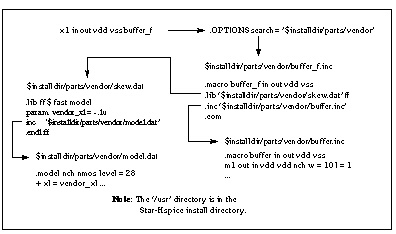
.OPTIONS SEARCH = `directory_path'

Example

.OPTIONS SEARCH = `$installdir/parts/vendor'

The above example sets the search path to find models by way of a vendor subdirectory under the installation directory, $installdir/parts (see Vendor Library Usage). The DDL subdirectories are contained in the parts/ directory.

Figure 3-2: Vendor Library Usage

Automatic Library Selection

Automatic library selection allows a search order for up to 40 directories. The hspice.ini file sets the default search paths. Use this file for any directories that should always be searched. Star-Hspice searches for libraries in the order in which libraries are specified in .OPTIONS SEARCH statements. When Star Hspice encounters a subcircuit call, the search order is as follows:

1. Read the input file for a .SUBCKT or .MACRO with call name.

2. Read any .INC files or .LIB files for a .SUBCKT or .MACRO with the call
name.

3. Search the directory that the input file was in for a file named call_name.inc .

4. Search the directories in the .OPTIONS SEARCH list.

By using the Star-Hspice library search and selection features you can, for example, simulate process corner cases, using .OPTIONS SEARCH = `<libdir>' to target different process directories. If you have an input/output buffer subcircuit stored in a file named iobuf.inc, create three copies of the file to simulate fast , slow and typical corner cases. Each file contains different Star-Hspice transistor models representing the different process corners. Store these files (all named iobuf.inc) in separate directories.

.PARAM Statement

Use the .PARAM statement to define parameters. Parameters in Star-Hspice are names that have associated numeric values. You can use any of the following methods to define parameters:

• Simple Parameter
• Algebraic Parameter
• .User-Defined Function
• Subcircuit Default Definition
• Predefined Analysis
• Measurement Parameters

Simple Parameter

A simple parameter assignment is a constant real number. The parameter keeps this value unless there is a later definition that changes its value, or it is assigned a new value by an algebraic expression during simulation. There is no warning if a parameter is reassigned.

Syntax

.PARAM (ParamName>=<RealNumber>

Algebraic Parameter

Algebraic parameter assignments can be made by an algebraic expression of real values, predefined function, user-defined function, or circuit or model values. A complex expression must be enclosed in single quotes to invoke the Star-Hspice algebraic processor unless the expression begins with an alphabetic character and contains no blank spaces. A simple expression consists of a single parameter name.

Syntax

.PARAM <ParamName>='<Expression>'

or

.PARAM <ParamName1>=<ParamName2>

To use an algebraic expression as an output variable in a .PRINT, .PLOT, or .PROBE statement, use the PAR keyword:

.PRINT DC v(3) gain=PAR(`v(3)/v(2)')
+ PAR(`V(4)/V(2)')

Example

.para x=cos(2)+sin(2)

.User-Defined Function

A user-defined function assignment is similar to the definition of an algebraic parameter definition. Star-Hspice extends the algebraic parameter definition to include function parameters that are used in the algebraic that defines the function.

User-defined functions cannot be nested more than three deep.

Syntax

.PARAM <ParamName>(<pv1>[<pv2>])='<Expression>'

Subcircuit Default Definition

The specification of hierarchical subcircuits allows you to pick default values for circuit elements. This is typically used in cell definitions so that the circuit can be simulated with typical values.

Syntax

.SUBCKT <SubName><PinList>[<SubDefaultsList>]

where SubDefaultsList is:

<SubParam1>=<Expression>[<SubParam1>=<Expression>...]

Predefined Analysis

Star-hspice has specialized analysis types, primarily Optimization and Monte Carlo, that require a method of controlling the analysis. The syntax for these uses of .PARAM are described in .PARAM Distribution Function Syntax.

Measurement Parameters

.MEASURE statements in Star-Hspice produce a type of parameter called a measurement parameter. In general, the rules for measurement parameters are the same as those for standard parameters with the exception of the definition: measurement parameters are not defined in a .PARAM statement but directly in the .MEASURE statement. For more information, see Measure Parameter Types.

.PROTECT Statement

Use the .PROTECT statement to keep models and cell libraries private. The .PROTECT statement suppresses the printout of the text from the list file, like the option BRIEF. The .UNPROTECT command restores normal output functions. In addition, any elements and models located between a .PROTECT and an .UNPROTECT statement inhibit the element and model listing from the option LIST. Any nodes that are contained within the .PROTECT and .UNPROTECT statements are not listed in the .OPTIONS NODE nodal cross reference, and are not listed in the .OP operating point printout.

Syntax

.PROTECT

.UNPROTECT Statement

The .UNPROTECT statement restores normal output functions from a .PROTECT statement. Any elements and models located between .PROTECT and .UNPROTECT statements inhibit the element and model listing from the option LIST. Any nodes contained within the .PROTECT and .UNPROTECT statements are not listed in either the .OPTIONS NODE nodal cross reference, or in the .OP operating point printout.

Syntax

.UNPROTECT

.ALTER Statement

You can use the .ALTER statement to rerun a simulation using different parameters and data.

Print and plot statements must be parameterized to be altered. The .ALTER block cannot include .PRINT, .PLOT, .GRAPH or any other input/output statements. You can include all analysis statements (.DC, .AC, .TRAN, .FOUR, .DISTO, .PZ, and so on) in only one .ALTER block in an input netlist file, but only if the analysis statement type has not been used previously in the main program. The .ALTER sequence or block can contain:

• Element statements (except source elements)
• .DATA statements
• .DEL LIB statements
• .INCLUDE statements
• .IC (initial condition) and .NODESET statements
• .LIB statements
• .MODEL statements
• .OP statements
• .OPTIONS statements
• .PARAM statements
• .TEMP statements
• .TF statements
• .TRAN, .DC, and .AC statements

Altering Design Variables and Subcircuits

The following rules are used when altering design variables and subcircuits.

1. If the name of a new element, .MODEL statement, or subcircuit definition
is identical to the name of an original statement of the same type, the new
statement replaces the old. New statements are added to the input netlist file.

2. Element and .MODEL statements within a subcircuit definition can be
changed and new element or .MODEL statements can be added to a
subcircuit definition. Topology modifications to subcircuit definitions
should be put into libraries and added with .LIB and deleted with .DEL LIB.

3. If a parameter name of a new .PARAM statement in the .ALTER module is
identical to a previous parameter name, the new assigned value replaces the old.

4. If elements or model parameter values were parameterized when using
.ALTER, these parameter values must be changed through the .PARAM
statement. Do not redescribe the elements or model parameters with
numerical values.

5. Options turned on by an .OPTION statement in an original input file or a
.ALTER block can be turned off.

6. Only the actual altered input is printed for each .ALTER run. A special
.ALTER title identifies the run.

7. .LIB statements within a file called with an .INCLUDE statement cannot be
revised by .ALTER processing, but .INCLUDE statements within a file
called with a .LIB statement can be accepted by .ALTER processing.

Using Multiple .ALTER Statements

For the first run, Star-Hspice reads the input file only up to the first .ALTER statement and performs the analyses up to that .ALTER statement. After the first simulation is completed, Star-Hspice reads the input between the first .ALTER and the next .ALTER or .END statement. These statements are then used to modify the input netlist file. Star-Hspice then resimulates the circuit.

For each additional .ALTER statement, Star-Hspice performs the simulation preceding the first .ALTER statement, then performs another simulation using the input between the current .ALTER statement and the next .ALTER statement or the .END statement. If you do not want to rerun the simulation preceding the first .ALTER statement every time, put the statements preceding the first .ALTER statement in a library and use the .LIB statement in the main input file, and put a .DEL LIB statement in the .ALTER section to delete that library.

Syntax

.ALTER <title_string>

The title_string is any string up to 72 characters. The appropriate title string for each .ALTER run is printed in each section heading of the output listing and the graph data (.tr#) files.

.DEL LIB Statement

The .DEL LIB statement is used with the .ALTER statement to remove library data from memory. The .DEL LIB statement causes the .LIB call statement with the same library number and entry name to be removed from memory the next time the simulation is run. A .LIB statement can then be used to replace the deleted library.

Syntax

.DEL LIB `<filepath>filename' entryname
.DEL LIB libnumber entryname

where:

Example

FILE1: ALTER1 TEST  CMOS INVERTER

.OPTIONS ACCT LIST

.TEMP 125

.PARAM WVAL = 15U VDD = 5

*

.OP

.DC VIN 0  5  0.1

.PLOT DC V(3) V(2)

*

VDD 1 0 VDD

VIN 2 0

*

M1  3  2  1  1  P 6U 15U

M2  3  2  0  0  N 6U W = WVAL

*

.LIB 'MOS.LIB' NORMAL

.ALTER

.DEL LIB 'MOS.LIB' NORMAL					$removes LIB from memory

$PROTECTION

.PROT 					$protect statements below .PROT

.LIB 'MOS.LIB' FAST 					$get fast model library

.UNPROT

.ALTER

.OPTIONS NOMOD OPTS				 	$suppress model parameters printing

* 				 	and print the option summary

.TEMP -50  0  50				 	$run with different temperatures

.PARAM WVAL = 100U VDD = 5.5	 				$change the parameters

VDD 1 0 5.5				 	$using VDD 1 0 5.5 to change the

				 	$power supply VDD value doesn't

					$work

VIN 2 0 PWL 0NS 0 2NS 5 4NS 0 5NS 5

				 	$change the input source

.OP VOL				 	$node voltage table of operating

				 	$points

.TRAN 1NS 5NS				 	$run with transient also

M2 3 2 0 0 N 6U WVAL				 	$change channel width

.MEAS SW2 TRIG V(3) VAL = 2.5 RISE = 1 TARG V(3)

+ VAL = VDD CROSS = 2 				 	$measure output

*

.END

Example 1 calculates a DC transfer function for a CMOS inverter. The device is first simulated using the inverter model NORMAL from the MOS.LIB library. By using the .ALTER block and the .LIB command, a faster CMOS inverter, FAST, is substituted for NORMAL and the circuit is resimulated. With the second .ALTER block, DC transfer analysis simulations are executed at three different temperatures and with an n-channel width of 100 µm instead of 15 µm. A transient analysis also is conducted in the second .ALTER block, so that the rise time of the inverter can be measured (using the .MEASURE statement).

This is a second example:

FILE2: ALTER2.SP CMOS INVERTER USING SUBCIRCUIT

.OPTIONS LIST ACCT

.MACRO INV 1 2 3

M1 3 2 1 1 P 6U 15U

M2 3 2 0 0 N 6U 8U

.LIB 'MOS.LIB' NORMAL

.EOM INV

XINV 1 2 3 INV

VDD 1 0 5

VIN 2 0

.DC VIN 0 5 0. 1

.PLOT V(3) V(2)

.ALTER

.DEL LIB 'MOS.LIB' NORMAL

.TF V(3) VIN $DC small-signal transfer function

*

.MACRO INV 1 2 3 $change data within subcircuit def

M1 4 2 1 1 P 100U 100U $change channel length,width,also

$topology

M2 4 2 0 0 N 6U 8U $change topology

R4 4 3 100 $add the new element

C3 3 0 10P $add the new element

.LIB 'MOS.LIB' SLOW $set slow model library

$.INC 'MOS2.DAT' $not allowed to be used inside

$subcircuit allowed outside

$subcircuit

.EOM INV

*

.END

In this example, the .ALTER block adds a resistor and capacitor network to the circuit. The network is connected to the output of the inverter and a DC small-signal transfer function is simulated.

.END Statement

The Star-Hspice input netlist file must have an .END statement as the last statement. The period preceding END is a required part of the statement.

Any text that follows the .END statement is treated as a comment and has no effect on that simulation. A Star-Hspice input file that contains more than one Star-Hspice run must have an .END statement for each Star-Hspice run. Any number of simulations may be concatenated into a single file.

Syntax

.END <comment>

Example

MOS OUTPUT

.OPTIONS NODE NOPAGE

VDS 3 0

VGS 2 0

M1 1 2 0 0 MOD1 L = 4U W = 6U AD = 10P AS = 10P

.MODEL MOD1 NMOS VTO = -2 NSUB = 1.0E15 TOX = 1000 UO = 550

VIDS 3 1

.DC   VDS 0 10 0.5    VGS 0 5 1

.PRINT DC I(M1) V(2)

.END MOS OUTPUT

MOS CAPS

.OPTIONS SCALE = 1U  SCALM = 1U WL ACCT

.OP

.TRAN .1 6

V1 1 0 PWL 0 -1.5V 6 4.5V 

V2 2 0 1.5VOLTS

MODN1 2 1 0 0 M  10 3

.MODEL M NMOS VTO = 1 NSUB = 1E15 TOX = 1000 UO = 800 LEVEL = 1
+	CAPOP = 2

.PLOT TRAN V(1) (0,5) LX18(M1)  LX19(M1) LX20(M1) (0,6E-13)

.END MOS CAPS