Star-Hspice Independent Source Functions

Star-Hspice provides the following types of independent source functions:

• Pulse (PULSE function)
• Sinusoidal (SIN function)
• Exponential (EXP function)
• Piecewise linear (PWL function)
• Single-frequency FM (SFFM function)
• Single-frequency AM (AM function)

PWL also comes in a data driven version. The data driven PWL allows the results of an experiment or a previous simulation to provide one or more input sources for a transient simulation.

The independent sources supplied with Star-Hspice permit the designer to specify a variety of useful analog and digital test vectors for either steady state, time domain, or frequency domain analysis. For example, in the time domain, both current and voltage transient waveforms can be specified as exponential, sinusoidal, piecewise linear, single-sided FM functions, or AM functions.

Pulse Source Function

Star-Hspice has a trapezoidal pulse source function, which starts with an initial delay from the beginning of the transient simulation interval to an onset ramp. During the onset ramp, the voltage or current changes linearly from its initial value to the pulse plateau value. After the pulse plateau, the voltage or current moves linearly along a recovery ramp, back to its initial value. The entire pulse repeats with a period per from onset to onset.

The general syntax for including a pulse source in an independent voltage or current source is:

General form:

Vxxx n+ n- PU<LSE> <(>v1 v2 <td <tr <tf <pw <per>>>>> <)>

or

Ixxx n+ n- PU<LSE> <(>v1 v2 <td <tr <tf <pw <per>>>>> <)>

The arguments are defined as:

Below is a table showing the time-value relationship for a PULSE source:

Intermediate points are determined by linear interpolation.

Example

The following example shows the pulse source connected between node 3 and node 0. The pulse has an output high voltage of 1 V, an output low voltage of -1 V, a delay of 2 ns, a rise and fall time of 2 ns, a high pulse width of 50 ns, and a period of 100 ns.

VIN 3 0 PULSE (-1 1 2NS 2NS 2NS 50NS 100NS)

Pulse source connected between node 99 and node 0. The syntax shows parameterized values for all the specifications.

V1 99 0 PU lv hv tdlay tris tfall tpw tper

This example shows an entire Star-Hspice netlist, which contains a PULSE voltage source. The source has an initial voltage of 1 volt, a pulse voltage of 2 volts, a delay time, rise time and fall time each of 5 nanoseconds, a pulse width of 20 nanoseconds, and a pulse period of 50 nanoseconds. The result of the simulation of this netlist is shown in Pulse Source Function.

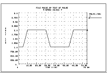
File pulse.sp test of pulse

.option post

.tran .5ns 75ns

vpulse 1 0 pulse( v1 v2 td tr tf pw per )

r1 1 0 1

.param v1=1v v2=2v td=5ns tr=5ns tf=5ns pw=20ns

+ per=50ns

.end

Figure 5-1: Pulse Source Function

Sinusoidal Source Function

Star-Hspice has a damped sinusoidal source that is the product of a dying exponential with a sine wave. Application of this waveform requires the specification of the sine wave frequency, the exponential decay constant, the beginning phase, and the beginning time of the waveform, as explained below.

The general syntax for including a sinusoidal source in an independent voltage or current source is:

General Form:

Vxxx n+ n- SIN <(> vo va <freq <td < < >>>> <)>

or

Ixxx n+ n- SIN <(> vo va <freq <td < < >>>> <)>

The arguments are defined as:

The waveform shape is given by the following table of expressions:

Time Value
0 to td
td to tstop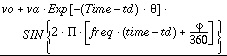

where TSTOP is the final time; see the .TRAN statement for a detailed explanation.

Example

VIN 3 0 SIN (0 1 100MEG 1NS 1e10)

Damped sinusoidal source connected between nodes 3 and 0. The waveform has a peak value of 1 V, an offset of 0 V, a 100-MHz frequency, a time delay of 1 ns, a damping factor of 1e10, and a phase delay of zero degree. See Sinusoidal Source Function for a plot of the source output.

Figure 5-2: Sinusoidal Source Function

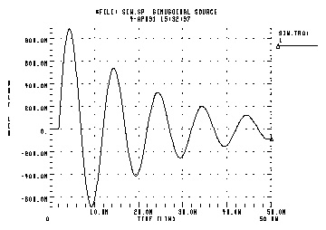
*File: SIN.SP THE SINUSOIDAL WAVEFORM

*<decay envelope>

.OPTIONS POST

.PARAM V0=0 VA=1 FREQ=100MEG DELAY=2N THETA=5E7

+ PHASE=0

V 1 0 SIN (V0 VA FREQ DELAY THETA PHASE)

R 1 0 1

.TRAN .05N 50N

.END

This example shows an entire Star-Hspice netlist that contains a SIN voltage source. The source has an initial voltage of 0 volts, a pulse voltage of 1 volt, a delay time of 2 nanoseconds, a frequency of 100 MHz, and a damping factor of 50 MHz.

Exponential Source Function

The general syntax for including an exponential source in an independent voltage or current source is:

General Form:

Vxxx n+ n- EXP <(> v1 v2 <td1 < 1 <td2 < 2>>>> <)>

or

Ixxx n+ n- EXP <(> v1 v2 <td1 < 1 <td2 < 2>>>> <)>

The arguments are defined as:

TSTEP is the printing increment, and TSTOP is the final time.

The waveform shape is given by the following table of expressions:

Time Value

0 to td1

td1 to td2

td2 to tstop

Example

VIN 3 0 EXP (-4 -1 2NS 30NS 60NS 40NS)

The above example describes an exponential transient source that is connected between nodes 3 and 0. It has an initial t=0 voltage of -4 V and a final voltage of -1 V. The waveform rises exponentially from -4 V to -1 V with a time constant of 30 ns. At 60 ns it starts dropping to -4 V again, with a time constant of 40 ns.

Figure 5-3: Exponential Source Function

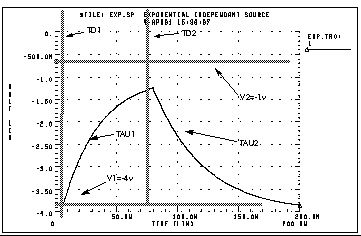
*FILE: EXP.SP THE EXPONENTIAL WAVEFORM

.OPTIONS POST

.PARAM V1=-4 V2=-1 TD1=5N TAU1=30N TAU2=40N TD2=80N

V 1 0 EXP (V1 V2 TD1 TAU1 TD2 TAU2)

R 1 0 1

.TRAN .05N 200N

.END

This example shows an entire Star-Hspice netlist that contains an EXP voltage source. It has an initial t=0 voltage of -4 V and a final voltage of -1 V. The waveform rises exponentially from -4 V to -1 V with a time constant of 30 ns. At 80 ns it starts dropping to -4 V again, with a time constant of 40 ns.

Piecewise Linear (PWL) Source Function

The general syntax for including a piecewise linear source in an independent voltage or current source is:

General Form:

Vxxx n+ n- PWL <(> t1 v1 <t2 v2 t3 v3...> <R <=repeat>>
+ <TD=delay> <)>

Or

Ixxx n+ n- PWL <(> t1 v1 <t2 v2 t3 v3...> <R <=repeat>>
+ <TD=delay> <)>

MSINC and ASPEC form:

Vxxx n+ n- PL <(> v1 t1 <v2 t2 v3 t3...> <R <=repeat>>
+ <TD=delay> <)>

Or

Ixxx n+ n- PL <(> v1 t1 <v2 t2 v3 t3...> <R <=repeat>>
+ <TD=delay> <)>

The arguments are defined as:

Each pair of values (t1, v1) specifies that the value of the source is v1 (in volts or amps) at time t1. The value of the source at intermediate values of time is determined by linear interpolation between the time points. ASPEC style formats are accommodated by the "PL" form of the function, which reverses the order of the time-voltage pairs to voltage-time pairs. Star-Hspice uses the DC value of the source as the time-zero source value if no time-zero point is given. Also, Star-Hspice does not force the source to terminate at the TSTOP value specified in the .TRAN statement.

If the slope of the piecewise linear function changes below a certain tolerance, the timestep algorithm may not choose the specified time points as simulation time points, thereby obtaining a value for the source voltage or current by extrapolation of neighboring values. In this situation, you may notice a small deviation of the simulated voltage from that specified in the PWL list. To force Star-Hspice to use the specified values, use the SLOPETOL option to reduce the slope change tolerance (see Specifying Simulation Outputfor more information about this option).

Specify "R" to cause the function to repeat. You can specify a value after this "R" to indicate the beginning of the function to be repeated: the repeat time must equal a breakpoint in the function. For example, if t1 = 1, t2 = 2, t3 = 3, and t4 = 4, "repeat" can be equal to 1, 2, or 3.

Specify TD=val to cause a delay at the beginning of the function. You can use TD with or without the repeat function.

Example

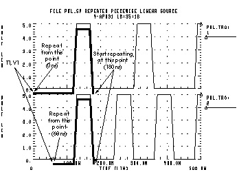
*FILE: PWL.SP THE REPEATED PIECEWISE LINEAR SOURCE

*ILLUSTRATION OF THE USE OF THE REPEAT FUNCTION "R"

*file pwl.sp REPEATED PIECEWISE LINEAR SOURCE

.OPTION POST

.TRAN 5N 500N

V1 1 0 PWL 60N 0V, 120N 0V, 130N 5V, 170N 5V, 180N 0V, R 0N

R1 1 0 1

V2 2 0 PL 0V 60N, 0V 120N, 5V 130N, 5V 170N, 0V 180N, R 60N

R2 2 0 1

.END

This example shows an entire Star-Hspice netlist that contains two piecewise linear voltage sources. The two sources have the same function (the first one is in normal format, and the second in ASPEC format). The first source has a repeat specified to start at the beginning of the function, whereas the second repeat starts at the first timepoint. See Results of Using the Repeat Function for the difference in responses.

Figure 5-4: Results of Using the Repeat Function

Data Driven Piecewise Linear Source Function

The general syntax for including a data-driven piecewise linear source in an independent voltage or current source is:

General Form:

Vxxx n+ n- PWL (TIME, PV)

or

Ixxx n+ n- PWL (TIME, PV)

along with:

.DATA dataname

TIME PV

t1 v1

t2 v2

t3 v3

t4 v4

.. ..

.ENDDATA

.TRAN DATA=datanam

The arguments are defined as:

TIME Parameter name for time value provided in a .DATA statement.

PV Parameter name for amplitude value provided in a .DATA statement.

You must use this source with a .DATA statement that contains time-value pairs. For each tn-vn (time-value) pair given in the .DATA block, the data driven PWL function outputs a current or voltage of the given tn duration and with the given vn amplitude.

This source allows you to use the results of one simulation as an input source in another simulation. The transient analysis must be data driven.

Example

*DATA DRIVEN PIECEWISE LINEAR SOURCE

V1 1 0 PWL(TIME, pv1)

R1 1 0 1

V2 2 0 PWL(TIME, pv2)

R2 2 0 1

.DATA dsrc

TIME pv1 pv2

0n 5v 0v

5n 0v 5v

10n 0v 5v

.ENDDATA

.TRAN DATA=dsrc

.END

This example shows an entire Star-Hspice netlist that contains two data-driven piecewise linear voltage sources. The .DATA statement contains the two sets of value data referenced in the sources, pv1 and pv2. The .TRAN statement references the data name.

Single-Frequency FM Source Function

The general syntax for including a single-frequency frequency-modulated source in an independent voltage or current source is:

General Form:

Vxxx n+ n- SFFM <(> vo va <fc <mdi <fs>>> <)>

or

Ixxx n+ n- SFFM <(> vo va <fc <mdi <fs>>> <)>

The arguments are as follows:

The waveform shape is given by the following expression:

Example

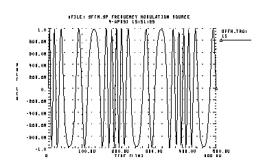
*FILE: SFFM.SP THE SINGLE FREQUENCY FM SOURCE

.OPTIONS POST

V 1 0 SFFM (0, 1M, 20K. 10, 5K)

R 1 0 1

.TRAN .0005M .5MS

.END

This example shows an entire Star-Hspice netlist that contains a single-frequency frequency-modulated voltage source. The source has an offset voltage of 0 volts, and a maximum voltage of 1 millivolt. The carrier frequency is 20 kHz, and the signal is 5 kHz, with a modulation index of 10 (the maximum wavelength is roughly 10 times longer than the minimum).

Figure 5-5: Single Frequency FM Source

Amplitude Modulation Source Function

The general syntax for including a single-frequency frequency-modulated source in an independent voltage or current source is:

General form:

Vxxx n+ n- AM < (> sa oc fm fc <td> <)>

or

Ixxx n+ n- AM < (> sa oc fm fc <td> <)>

The arguments are as follows:

where

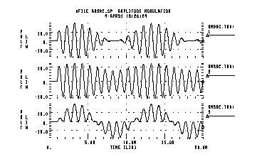
The waveform shape is given by the following expression:

Example

.OPTION POST

.TRAN .01M 20M

V1 1 0 AM(10 1 100 1K 1M)

R1 1 0 1

V2 2 0 AM(2.5 4 100 1K 1M)

R2 2 0 1

V3 3 0 AM(10 1 1K 100 1M)

R3 3 0 1

.END

This example shows an entire Star-Hspice netlist that contains three amplitude-modulated voltage sources. The first has an amplitude of 10, an offset constant of 1, a carrier frequency of 1 kHz, a modulation frequency of 100 Hz, and a delay of 1 millisecond. The second source has the same frequencies and delay, but with an amplitude of 2.5 and an offset constant of 4. The third source is the same as the first but with the carrier and modulation frequencies exchanged.

Figure 5-6: Amplitude Modulation Plot